This is a project I completed based on the Climate Change AI Summer School 2023 Tutorial of the same name. You can find the original here: Predicting Mobility Demand from Urban Features Tutorial
Overview
Goal
Investigate the relationship between points-of-interest densities and bike-sharing demand using linear regression and graph neural networks.
Motivation
Knowing the demand for shared bikes at different locations and different times will allow cities to ensure that there are enough available bikes, incentivizing citizens to use bikes over more polluting forms of transportation It can also help inform city planners on where to put new bike sharing stands.
Dataset
Data
- Shape files specifying locations (latitude/longitude coordinates) of the points-of-interest (restaurants, hospital, bus stops, etc)
- Trip (start and end points) Data from 2021
- Shape files for Shenzhen, Shenzhen’s population distribution, Shenzhen’s bus/metro stops The data can be accessed here: https://drive.google.com/drive/u/3/folders/18bdGh6IIRhqKr3gPQhbuhkOgZykBrfqx
Preprocessing
We load a single CSV into a pandas dataframe like this, taking only 100,000 random samples out of the 10 million:
df = pd.read_csv('/content/data/Shenzhen Bike-Share Data/8.01-8.30/shared_bike_data/21_1000w.csv')
df = df.sample(100000).reset_index(drop=True)
We then filter out data that lies outside Shenzhen by getting only the approximate rectangle (in lat/long coordinates):
# selecting approx coordinates around Shenzhen
longitude_range = [113.7, 114.7]
latitude_range = [22.0, 23.0]
col_to_range_map = {"START_LAT" : latitude_range,
                    "START_LNG" : longitude_range,
                    "END_LAT" : latitude_range,
                    "END_LNG" : longitude_range
                    }
for col, distance in col_to_range_map.items():
    df.drop(df[(df[col] > distance[1]) | (df[col] < distance[0])].index, inplace=True)
pd.DataFrame({
    'count': df.count(),
    'min': df.min(),
    'max': df.max()
})
#Convert the start and end time columns in the data frame to datetime objects
df['START_TIME'] = pd.to_datetime(df['START_TIME'])
df['END_TIME'] = pd.to_datetime(df['END_TIME'])
# add a column for whether a trip occurs on a weekday/weekend
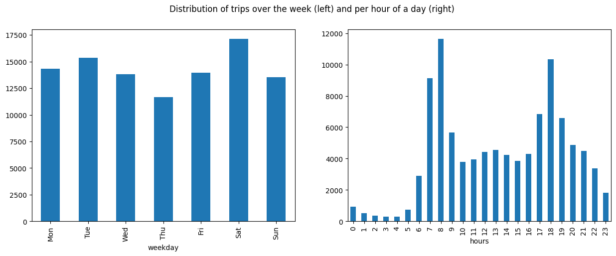
df.loc[:, 'IS_WEEKDAY'] = df['START_TIME'].dt.dayofweek < 5We also take a look at the temporal distribution of the trips:
weekday_names = {0:'Mon',1:'Tue',2:'Wed',3:'Thu',4:'Fri',5:'Sat',6:'Sun',}
order = weekday_names.values()

df['weekday'] = df['START_TIME'].dt.dayofweek
df['weekday'] = df['weekday'].replace(weekday_names)
df['hours'] = df['START_TIME'].dt.hour

weekdays = df.groupby('weekday').size().to_frame('count').loc[order].reset_index()
hours = df.groupby('hours').size().to_frame('count').reset_index()

fig,ax = plt.subplots(ncols=2, figsize=(15,5))
weekdays.plot.bar(ax=ax[0], x='weekday',y='count',legend = False)
hours.plot.bar(ax=ax[1], x='hours',y='count',legend=False)
plt.suptitle('Distribution of trips over the week (left) and per hour of a day (right)')
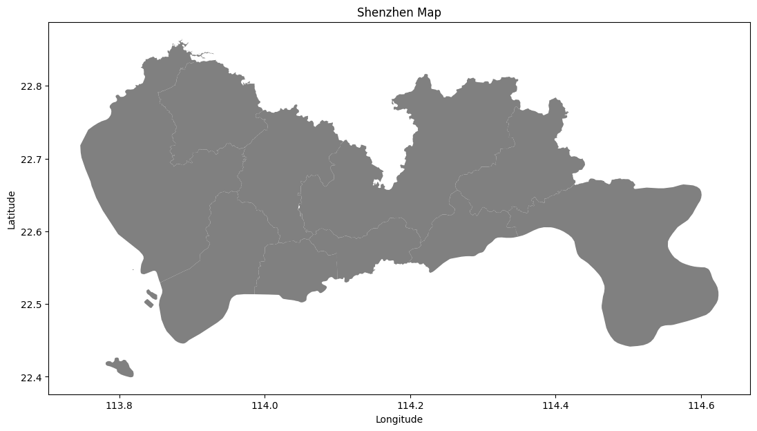
Visualizing the shape files:
shenzhen = gpd.read_file("data/Shenzhen Bike-Share Data/shenzhen/shenzhen.shp")
# Visualize
fig,ax = plt.subplots(figsize=(15,7))
shenzhen.plot(ax=ax,color='gray')
ax.set_title('Shenzhen Map')
ax.set_xlabel("Longitude")
ax.set_ylabel("Latitude")
We then plot the trip starting points and ending points on the map. These are the shared bike stands that people are retrieving/returning their bikes.
This can be done by creating geo-dataframes for both the start/end points.
# Create geopandas dataframes for start and end points separately
gdf_start = gpd.GeoDataFrame(df, geometry=[Point(xy) for xy in zip(df['START_LNG'], df['START_LAT'])],crs=4326)
gdf_end = gpd.GeoDataFrame(df, geometry=[Point(xy) for xy in zip(df['END_LNG'], df['END_LAT'])],crs=4326)
# Visualize Starting Locations
fig,ax = plt.subplots(ncols=2,figsize=(15,7))
shenzhen.plot(ax=ax[0],color='gray')
gdf_start.sample(10000).plot(ax=ax[0],color='blue',marker='o',markersize=0.001)
ax[0].set_title('Starting Locations')
ax[0].set_axis_off()

shenzhen.plot(ax=ax[1],color='gray')
gdf_end.sample(10000).plot(ax=ax[1],color='red',marker='o',markersize=0.001)
ax[1].set_title('Ending Locations')
ax[1].set_axis_off()
To get the points-of-interest on the map, it’s the same process:
# Set path to shapefile directory
poi_dir_path = '/content/data/Shenzhen Bike-Share Data/ShenzhenPOI/ShapeFile'

# Load poi shape files
shp_files = []
for file_path in os.listdir(poi_dir_path):
  if file_path.endswith(".shp"):
    for cat in poi_cat:
      if cat in file_path:
        shp_file = gpd.read_file(os.path.join(poi_dir_path, file_path))
        shp_file['POI_TYPE'] = cat
        shp_files.append(shp_file)
        continue
# Create geo dataframe from all POIs
poi_gdf = pd.concat(shp_files).pipe(gpd.GeoDataFrame)
poi_gdf.describe(include='all')
# save the gdf
poi_gdf.to_file(compiled_poi_path + '/compiled.shp', encoding='UTF-8')
Methods
Now, let’s try to see how the trip start/end locations and their frequency are correlated with the points-of-interest.
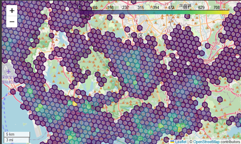
We use the [h3pandas](H3-Pandas — h3pandas 0.1 documentation) library from Uber to create a hexagonal grid on the map and to count the number of trips ending in each grid cell.
import h3pandas

# Convert trip DataFrame to a GeoDataFrame with the geometry describing the trip destination
gdf = gpd.GeoDataFrame(df, crs='EPSG:4326', geometry=gpd.points_from_xy(df['END_LNG'], df['END_LAT']))

# Create a hexagonal grid using Uber's H3 library and count the number of trips ending in each grid cell
trips = gdf[['_id', 'geometry']].h3.geo_to_h3_aggregate(resolution=8, operation='count')
trips = trips.rename(columns={'_id': 'count'})

# Visualize trip destinations
trips.explore('count')
Let’s naively assume that the relationship is linear. Let’s use sklearn’s linear_model for each location in the grid.
for poi_type in ['SportsRecreation', 'TransportationService', 'MedicalService']:
    y = trips['count']
    X = trips[[poi_type]]

    # Perform linear regression
    lm = LinearRegression()
    lm.fit(X, y)

    # Print the results
    print(poi_type)
    print(f'Coefficients: {lm.coef_[0]:.1f}')
    print(f'Intercept: {lm.intercept_:.1f}')
    print(f'R-squared: {lm.score(X, y):.3f}')
    print()
SportsRecreation
Coefficients: 3.6
Intercept: 31.8
R-squared: 0.324

TransportationService
Coefficients: 2.8
Intercept: 9.6
R-squared: 0.402

MedicalService
Coefficients: 2.5
Intercept: 31.7
Combining for all categories of points-of-interest:
X = trips[['SportsRecreation', 'TransportationService', 'MedicalService']]
y = trips['count']

# Perform linear regression
lm = LinearRegression()
lm.fit(X, y)
y_pred_lm = lm.predict(X)

print(f'Coefficients: {lm.coef_}')
print(f'Intercept: {lm.intercept_:.1f}')
print(f'R-squared: {lm.score(X, y):.3f}')
Coefficients: [ 1.30159506 2.23879164 -0.18091492]
Intercept: 10.8
R-squared: 0.415
Let’s try using Gradient boosting decision trees instead
model = XGBRegressor()
model.fit(X, y)
y_pred_xgb = model.predict(X)

r2 = r2_score(y, y_pred_xgb)
print(f'R-squared: {r2:.3f}')
>>> R-squared: 0.964
This is great! But can we do better? There are clear spatial patterns in the bike trips, so we want a model that can learn from spatial dependencies. This brings us to:
GNNs
Constructing the Graph
We use the pytorch geometric library to generate a k-nearest neighbors graph. In this case, each node is a grid cell that is connected to 5 of its closest grid cells.
from torch_geometric.nn import knn_graph
from torch_geometric.data import Data
from torch_geometric.nn import GCNConv, GATConv, SAGEConv
import torch
import torch.nn as nn
import torch.utils.data
import torch.nn.functional as F

c = trips.geometry.centroid.get_coordinates()
X = trips[['SportsRecreation', 'TransportationService', 'MedicalService']]
y = trips['count']

# Convert to PyTorch data format
c_tensor = torch.tensor(c.values, dtype=torch.float)
X_tensor = torch.tensor(X.values, dtype=torch.float)
y_tensor = torch.tensor(y.values, dtype=torch.float)

# Determine neighboring grid cells
k = 5
edge_index = knn_graph(c_tensor, k=k, loop=False)

graph_data = Data(x=X_tensor, y=y_tensor, edge_index=edge_index, pos=c_tensor)
Architecture
class GCN(nn.Module):
    """
        A simple GCN with two convolutional layers
    """
    def __init__(self, num_features_in=3, num_features_out=1, hidden_dim=32, dropout=False):
        super(GCN, self).__init__()
        self.conv1 = GCNConv(num_features_in, hidden_dim)
        self.conv2 = GCNConv(hidden_dim, hidden_dim)
        self.fc = nn.Linear(hidden_dim, num_features_out)
        self.dropout = dropout

    def forward(self, x, edge_index):
        x = x.float()
        h1 = F.relu(self.conv1(x, edge_index))
        if self.dropout:
          h1 = F.dropout(h1, training=self.training)
        h2 = F.relu(self.conv2(h1, edge_index))
        if self.dropout:
          h2 = F.dropout(h2, training=self.training)
        output = self.fc(h2)
        return output
Training
lr = 1e-2
n_epochs = 1000
print_freq = 100

model = GCN(num_features_in=3, num_features_out=1, hidden_dim=32, dropout=False)
loss_fun = nn.MSELoss()
optimizer = torch.optim.AdamW(model.parameters(), lr=lr)

# Training loop
it_counts = 0
for epoch in range(n_epochs):
  it_counts += 1
  model.train()
  out = model(graph_data.x.float(), graph_data.edge_index)
  optimizer.zero_grad()
  loss = loss_fun(graph_data.y.float().reshape(-1), out.reshape(-1))
  loss.backward()
  optimizer.step()
  if it_counts % print_freq == 0:
    print(f'Loss: {loss.item():.1f}')
with torch.no_grad():
  model.eval()
  y_pred_gnn = model(graph_data.x.float(), graph_data.edge_index)

gnn_r2 = r2_score(graph_data.y, y_pred_gnn)
print(f'GNN R-squared: {gnn_r2:.3f}')
References
Wagner, F., Nachtigall, F., Rahman, S., & Klemmer, K. (2024). Predicting Mobility Demand from Urban Features [Tutorial]. In Climate Change AI Summer School. Climate Change AI. https://doi.org/10.5281/zenodo.11619223
Code Link: https://colab.research.google.com/drive/1GKAHGoJbVSLhs6SrBD1IiFwNAC-tSiC7?usp=sharing