GraphCast

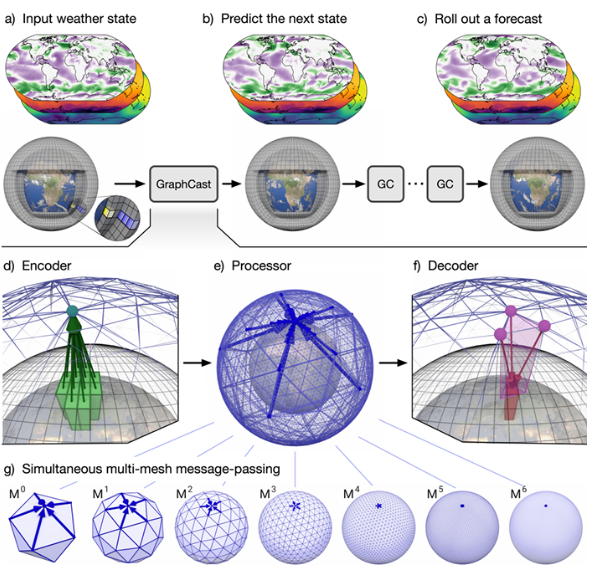
Introduction

Why AI-based weather forecasting?

Numerical weather prediction is computationally expensive and time-consuming.  

Graph

To start with building up the graph, we define the TypedGraph data structure. This is a graph made of a context (a class that indicates the number of graphs and the global features), as well as multiple sets of nodes and edges connecting those sets of nodes.

 
class TypedGraph(NamedTuple):
 
    """A graph with typed nodes and edges.
 
  
 
    A typed graph is made of a context, multiple sets of nodes and multiple
 
    sets of edges connecting those nodes (as indicated by the EdgeSetKey).
 
    """
 
  
 
    context: Context
 
    nodes: Mapping[str, NodeSet]
 
    edges: Mapping[EdgeSetKey, EdgeSet]
 
  
 
    def edge_key_by_name(self, name: str) -> EdgeSetKey:
 
        found_key = [k for k in self.edges.keys() if k.name == name]
 
        if len(found_key) != 1:
 
            raise KeyError("invalid edge key '{}'. Available edges: [{}]".format(
 
                    name, ', '.join(x.name for x in self.edges.keys())))
 
        return found_key[0]
 
  
 
    def edge_by_name(self, name: str) -> EdgeSet:
 
        return self.edges[self.edge_key_by_name(name)]
 

Loss Function

Variables

• $\tau \in 1:T_{\text{train}}$ are the lead times that correspond to the $T_{\text{train}}$ autoregressive steps.

• $d_0\in D_{\text{batch}}$ represent forecast initialization date-times in a batch of forecasts in the training set.

• $j\in J$ indexes the variable, and for atmospheric variables the pressure level.  

  E.g., $J=\{z_{1000},z_{850},\dots ,2T,\text{MSL}\}$.

• $i\in G_{0.25^{\circ }}$ are the location (latitude and longitude) coordinates in the grid.

• ${\hat{x}}_{j,i}^{d_0+\tau }$ and $x_{j,i}^{d_0+\tau }$ are predicted and target values for some variable-level, location, and lead time.

• $s_j$ is the per-variable-level inverse variance of time differences.

• $w_j$ is the per-variable-level loss weight.

• $a_i$ is the area of the latitude-longitude grid cell, which varies with latitude and is normalized to unit mean over the grid.

What is the per-variable-level inverse variance of time differences?

The inverse of the variance of the time differences for each variable; this is used to weight the loss for each variable.

To get a single scalar loss, they take the average of the losses across latitude/longitude, lead times, and batch size.

 
  
 
def weighted_mse_per_level(
 
    predictions: xarray.Dataset,
 
    targets: xarray.Dataset,
 
    per_variable_weights: Mapping[str, float],
 
) -> LossAndDiagnostics:
 
  """Latitude- and pressure-level-weighted MSE loss."""
 
  def loss(prediction, target):
 
    loss = (prediction - target)**2
 
    loss *= normalized_latitude_weights(target).astype(loss.dtype)
 
    if 'level' in target.dims:
 
      loss *= normalized_level_weights(target).astype(loss.dtype)
 
    return _mean_preserving_batch(loss)
 
  
 
  losses = xarray_tree.map_structure(loss, predictions, targets)
 
  return sum_per_variable_losses(losses, per_variable_weights)
 

The loss function is the MSE loss, but it is weighted by the latitude and pressure level. The normalized_latitude_weights and normalized_level_weights functions are used to calculate the weights for each latitude and pressure level.

Specifically, normalized_latitude_weights are proportional to the pressure at each level and the normalized_level_weights are proportional to (an approximation of) the grid cell area. The latter is done through some cosine/sine math.

References

The paper can be found here.

The code is provided by the authors of the paper. You can find the code here.